Fair samples from uneven workers

sample in APL has been a filter since 2023, and a good one. You give it a probability, it's pushed down into the block scans, and each row survives with that chance. For a quick look at a dataset it does exactly what you want.

What it can't do is count. A filter decides about each row on its own, with no idea how many rows came before or how many are left, so it can't promise you exactly 20 rows spread over a range. That's what people asked for, and it's what an agent pulling a handful of events into its context needs too.

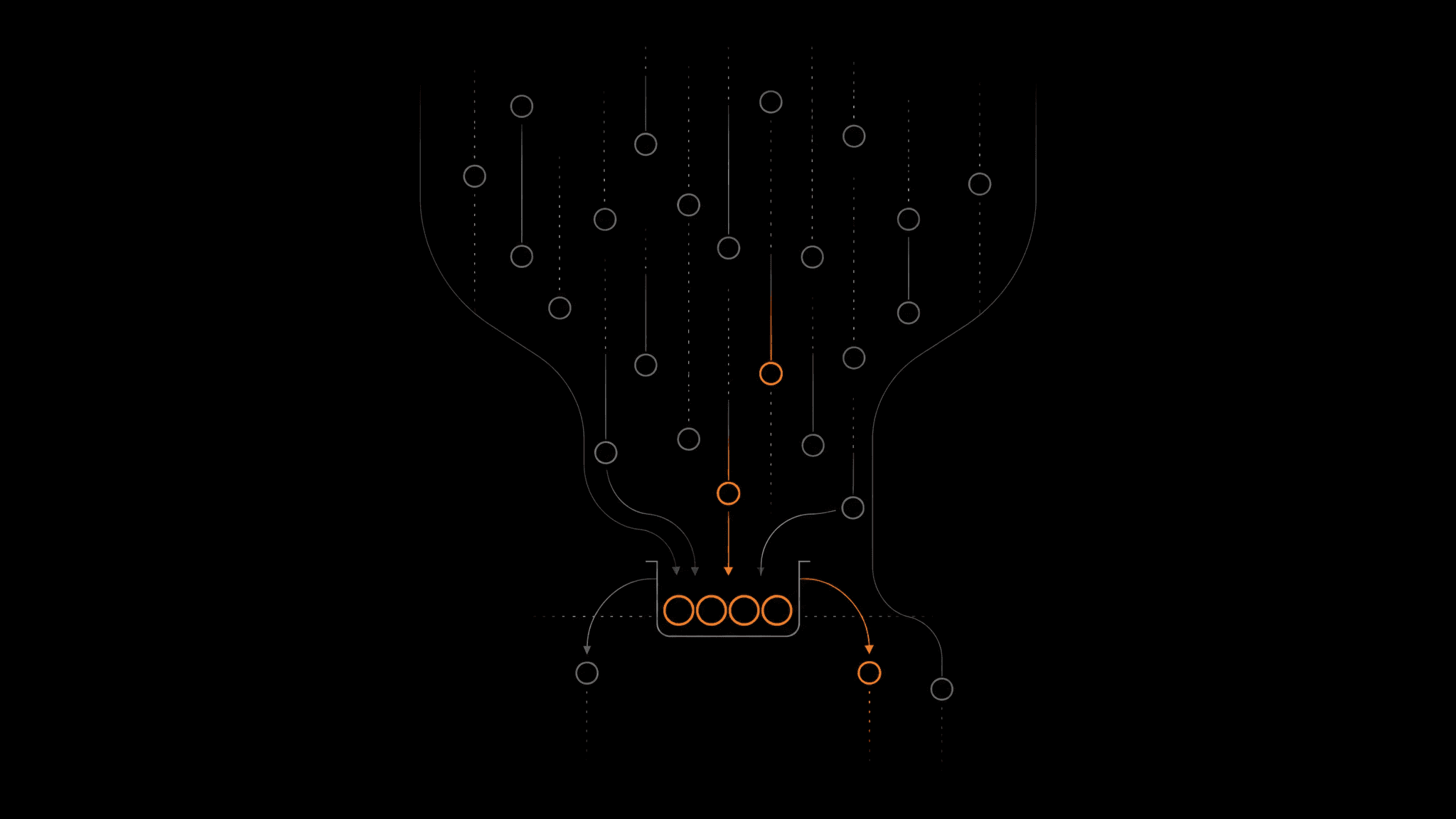
This is the story of sample n: an operator that returns n rows drawn uniformly from everything a query matched, and the merge that keeps it uniform when the query is spread across many workers. It took three pieces of work: the operator itself, making a random operator get along with the query cache, and teaching the distributed planner that equal-sized samples don't stand for equal amounts of data.

A filter can't count

Until now, the way to ask for 20 random rows was to combine the filter with a limit:

APL

['logs']
| where status >= 500
| sample 0.05
| take 20

take 20 ends the query as soon as 20 rows have made it through the filter. That's what makes it cheap, and it's also why the 20 rows come from whichever blocks the engine read first. The rest of the time range is never scanned.

We ran the same query on an hour of our own staging traces, against 5,122 spans with an HTTP status of 500 or higher. In three runs, sample 0.05 | take 20 returned all 20 rows from one five-minute interval and read at most 15% of the hour's rows. The interval at 08:45 held 44% of those errors and contributed none.

Filter sampling['logs'] | where status >= 500 | sample 0.05 | take 20

kept · rnd < 0.05scanned, droppednever scanned

To get n rows from the whole range, something has to see the whole range and keep state while it does. That's an operator, not a filter.

Algorithm R, one morsel at a time

Our query engine moves data between operators in chunks we call morsels, and we're moving every operator to work on them as they arrive rather than buffer everything first. Reservoir sampling fits that model well. We used the classic version, Algorithm R:

Keep a reservoir of n slots.
The first n matching rows go straight in.
The i-th matching row after that replaces a randomly chosen slot with probability n / i.

APL

['logs']
| where status >= 500
| sample 20

Algorithm R gives us two wins:

Constant memory usage: We don’t need to buffer all N matched rows in memory or know the total number of matches upfront. This makes Algorithm R a great fit for sampling n items from a stream of unknown length while keeping only a reservoir of size n. Memory usage stays at n rows regardless of how many rows match.
Uniform sampling: The way the algorithm decides whether to include a new row and which existing row to evict from the reservoir guarantees that every matched row has an equal probability of being selected: $n / N$ , where $N$ is the total number of matched rows across the entire range (assuming $N \ge n$ ).
Early rows are more likely to be pushed out as new rows arrive, while late rows are less likely to make it into the reservoir in the first place. These two effects balance out, giving every row the same chance of being included in the final sample.

Reservoir sampling['logs'] | where status >= 500 | sample 10

P(row ends in sample) · 4,000 replaysn / N = 10 / 120

Splitting a query splits the population

Large queries don't run on a single machine. The planner splits the scan across remote workers, each reading its own share of the blocks, while a local stage merges their results.

For most operators, the local stage is just a generic merge. When sample n first shipped, it got that generic merge too: each worker ran its own reservoir sampling and sent back up to N rows, and the coordinator combined them.

With four workers, that meant getting 80 rows back for a sample 20.

There are two problems with that:

We're getting more rows than we asked for. We need 20 rows, not 80. An easy fix would be to run the sampling algorithm again on those 80 rows, picking 20 out of them. Sounds good, right? Well, now we've introduced the second problem.
Those reservoirs don't represent the same amount of data. One worker might match 5,000 rows while another matches only 200, yet both send back 20 rows. Running the same sampling algorithm again on the combined 80 rows treats both reservoirs equally, even though the rows had very different chances of being selected in the first place.
For example, let's take two rows:
- Row a comes from a worker that matched 200 rows, so its chance of making it into that worker's reservoir is $20/200$ .
- Row b comes from a worker that matched 5,000 rows, so its chance is $20/5000$ .
Now, when we sample 20 rows from the combined 80, each returned row has another $20/80$ chance of being selected.
That gives us:
- Row a: $20/200 \times 20/80 = 1/40$
- Row b: $20/5000 \times 20/80 = 1/1000$
So row a is 25 times more likely to make it into the final sample than row b, simply because it came from a worker that matched fewer rows.
Doesn't seem super fair.

Weighting each reservoir by the rows it matched

The design for the fix started from a simple picture. Put every row the query matched in one box, colored by the worker that matched it. A fair sample of n rows is n balls drawn from that box without replacement. Counting the colors in that draw tells you how many rows each worker should contribute.

That draw is a "hypergeometric" draw, and it only needs one number from each worker: how many rows its reservoir was drawn from. Each reservoir now reports the rows presented to the sampler rather than the n it kept. The merge stage, SampleMerge, uses the counts in two steps:

Draw how many of the final n places each worker gets.
Fill each worker's places by picking that many rows uniformly from its reservoir.

The original design weighted by rows examined.

Wiring this in made sample the first operator the planner splits into a dedicated pair, a reservoir on each worker and a weighted merge on the coordinator. With n = 4, the plan looks like this:

text

local:  sample-merge[N=4]
remote: sample[N=4]

We ran the real operators 2,000 times with four workers and $n = 20$ :

Worker	Rows matched	True share	Weighted merge	Generic merge
A	5,000	62.5%	62.7%	25%
B	2,000	25%	24.6%	25%
C	800	10%	10.2%	25%
D	200	2.5%	2.5%	25%

Weighted merge['logs'] | where status >= 500 | sample 20

workers scan in parallel · each keeps a reservoir of n=20

worker A · 5,000 rowsworker B · 2,000 rowsworker C · 800 rowsworker D · 200 rows

“2,000 runs” measured with the real operators, four workers, n = 20, same rows matched

The math

Take a row on worker $i$ , which matched $N_i$ of the query's $T$ matching rows:

T = \sum_i N_i

The reservoir keeps it with probability $n/N_i$ . The merge gives worker $i$ a count $c_i$ of rows to fill and picks the row with probability $c_i / n$ :

P(\text{kept}) = \frac{n}{N_i}

c_i \sim \mathrm{Hypergeometric}(T,\ N_i,\ n), \qquad \mathbb{E}[c_i] = \frac{n\,N_i}{T}

Where we can see that $\mathbb{E}[c_i] = \frac{n\,N_i}{T}$ , with $d_j$ the $j$ -th of the $n$ draws, as follows:

c_i = \sum_{j=1}^{n} \mathbf{1}[\,d_j \in \text{worker } i\,]

P(d_j \in \text{worker } i) = \frac{N_i}{T}

\mathbb{E}[c_i] = \sum_{j=1}^{n} P(d_j \in \text{worker } i) = n \cdot \frac{N_i}{T}

P(\text{picked} \mid \text{kept}) = \frac{c_i}{n}

P(\text{row}) = \frac{n}{N_i} \cdot \frac{\mathbb{E}[c_i]}{n} = \frac{\mathbb{E}[c_i]}{N_i} = \frac{n}{T}

$N_i$ cancels out, so every matched row has the same $n/T$ chance, whichever worker read it.

This holds on average. Exact uniformity in every result was never the goal. Any single sample of 20 can still give a service, time interval or worker a little more or less than its share, the same way twenty coin flips rarely land ten and ten.

What this taught us

A filter and an operator answer different questions. A probability filter is cheap and stateless, and that's why it can't count. Once the question became "exactly N rows from everything", the answer had to be an operator with state.

Counters are part of the contract. Passing upstream status through the sampler looked like housekeeping. It ended up being the input the distributed merge depends on.

What's next

Today the weighting applies to a query over one dataset. The planner doesn't yet push sample through a union of several datasets, where internal row limits can cut each side short before it reaches a reservoir. And sample N still reads every matching row: the reservoir bounds memory and network traffic, not the scan, so skipping blocks while keeping the sample fair is the next thing to work on.

In the meantime, asking for 50 errors from last week gets you 50 errors from across last week, whether you're reading them or an agent is. Because we keep event history in the normal query path, that sample comes from everything you kept. The sample operator reference covers both forms.